Lily Samoyan

Portfolio of an Engineer of all trades
Low Power ML Hydrophones
Unfortunately, I am unable to share any of the data I worked with. I can share the results and code used for data analytics.
Project Purpose:
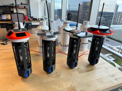
- Build out 5 ready for deployment AI Sonobuoys.
- Determine best solar panel and solar cap solution.
- Determine best SATCOMM antenna solution.
- Document the process.
Components:
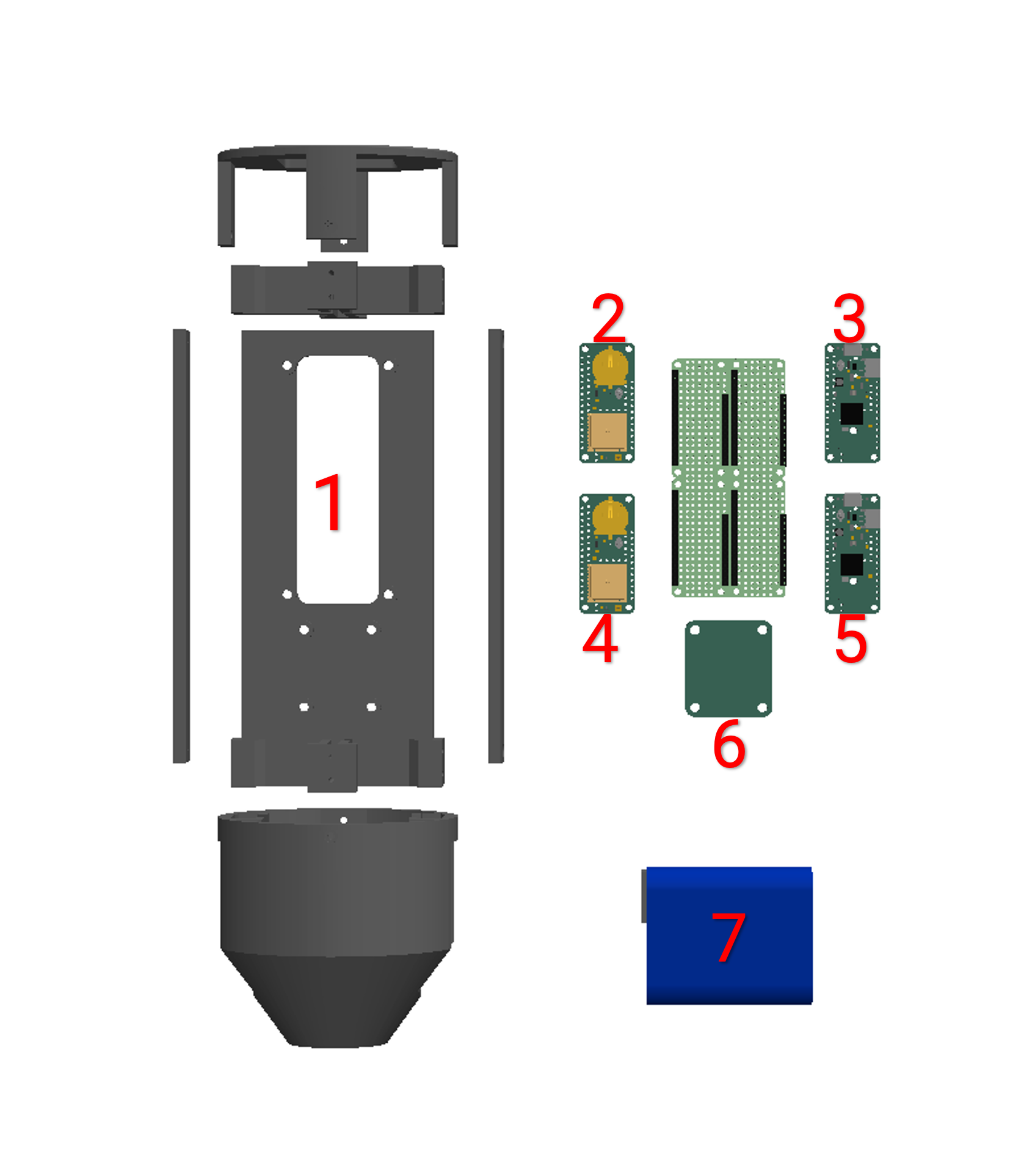
- Structural:
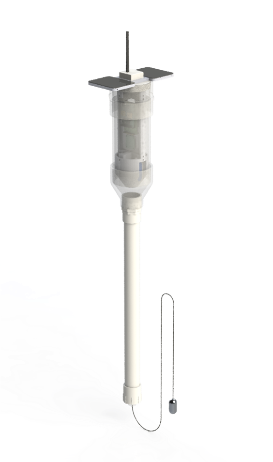
- Sonobuoy 3D Printed Housing
- PVC Piping Exterior
- Antenna
- Ground Plate
- Electronics:
- Particle Boron - Flashed
- Adafruit M4
- Myriota Module - Flashed
- SD Card Holder
- Solar Charger
- LiPo Battery
Base Assembly:
- Printed and assembled the 3D printed into the skeleton that will contain all of the electronics for each of the new buoys.
- Flashed the Particle Boron with the correct signal processing path.
- Flashed the Myriota Module with the correct transmit path to the Myriota dashboard to collect all data, which included battery percentage, buoy location, and associated times.
Prototyping/Design:
- Tested two different solar panels, one 4.8 V and one larger 6 V.
- The 6 V solar panels were able to hit the activation current of the solar charger more frequently, and thus was a better choice for the project.
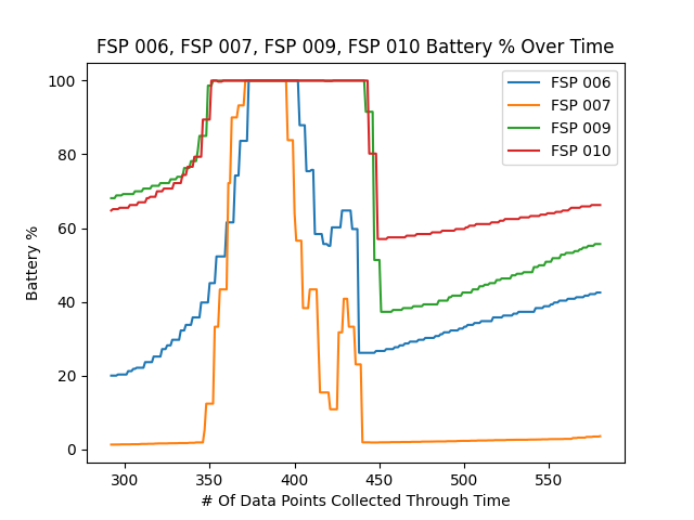
- Designed 4 different solar panel cap configurations with the 6 V solar panels and graphed the results of each cap version against each other. Then calculated the battery drop across all four configurations. The lowest would be the best bet, as it decreased battery decline by the most.
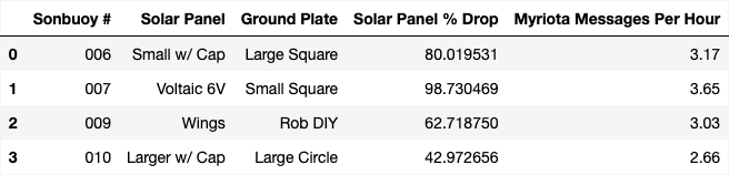
- The larger panels on a wider cap were a better choice with a 42% drop. The results for all the testing can be seen at the bottom of this page in results.
- Tested 4 different types of ground planes with a 433 MHz antenna to communicate with the Iridium network. The options were different sizes of squares, a small circle, and a ground plate with copper four copper wires. Found the number of packets/messages sent per hour for each ground plate.
- The small square cap was the best option. This is due to antenna theory, which states that the ground plane for signal reflection should have a diameter of pi/4 times the wavelength of the signal. This signal broadcasts at ~70cm, meaning a ground plane with a diameter of ~50 cm or 2 inches would be sufficient and ideal.
Results:
All 5 buoys were built out, with the testing being completed for the solar cap and antenna design. A table with more statistical data can be seen below. Additionally, at the bottom of this page all code will be pasted from data analysis ran on the code, with sensitivities removed.
Jupyter Notebook > Script
import pandas as pd
import numpy as np
from matplotlib import pyplot as plt
import dataframe_image as dfi
reference = pd.DataFrame()
reference["Sonbuoy #"] = ["006", "007", "009", "010"]
reference["Solar Panel"] = ["Small w/ Cap", "Voltaic 6V", "Wings","Larger w/ Cap"]
reference["Ground Plate"]= ["Large Square", "Small Square", "Rob DIY", "Large Circle"]
df = pd.read_csv()
df["FSP 006"].fillna(method="ffill", inplace=True)
df["FSP 007"].fillna(method="ffill", inplace=True)
df["FSP 009"].fillna(method="ffill", inplace=True)
df["FSP 010"].fillna(method="ffill", inplace=True)
df = df.drop(labels=[0, 1, 2], axis=0)
quarter = int((len(df["FSP 006"]))/4)
df1 = df[0:quarter]
df2 = df[quarter:2*quarter]
df3 = df[quarter*2:quarter*3]
df4 = df[quarter*3:-1]
type(df["FSP 006"][3])
plt.plot(df1["FSP 006"])
plt.plot(df1["FSP 007"])
plt.plot(df1["FSP 009"])
plt.plot(df1["FSP 010"])
plt.plot(df2["FSP 006"], label="FSP 006")
plt.plot(df2["FSP 007"], label="FSP 007")
plt.plot(df2["FSP 009"], label="FSP 009")
plt.plot(df2["FSP 010"], label="FSP 010")
plt.title("FSP 006, FSP 007, FSP 009, FSP 010 Battery % Over Time")
plt.xlabel("# Of Data Points Collected Through Time")
plt.ylabel("Battery %")
plt.legend(loc="best")
plt.savefig('006 vs 007 vs 009 vs 010 Battery.png')
mins = [ df2["FSP 006"].min(), df2["FSP 007"].min(), df2["FSP 009"].min(), df2["FSP 010"].min() ]
maxminlist = []
for i in range(len(mins)):
randovar = 100 - mins[i]
maxminlist.append(randovar)
reference["Solar Panel % Drop"] = maxminlist
reference
m07 = pd.read_csv()
m06 = pd.read_csv()
m09 = pd.read_csv()
m10 = pd.read_csv()
buck06 = len(m06['location'])
buck07 = len(m07['location'])
buck09 = len(m09['location'])
buck10 = len(m10['location'])
tot = buck06+buck07+buck09+buck10
print(buck07/tot, tot)
sizes = [buck06, buck07, buck09, buck10]
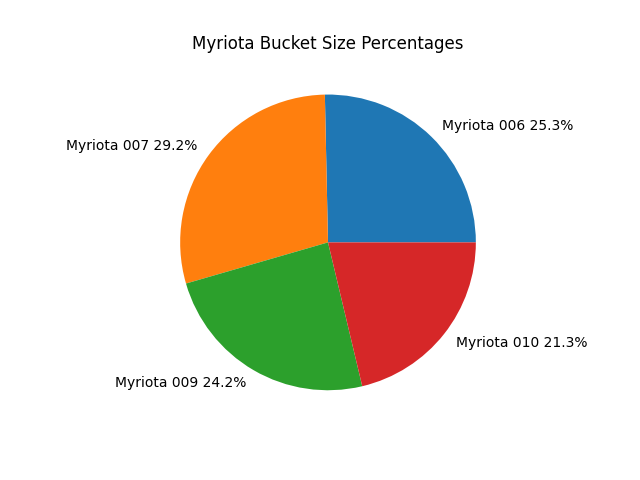
labels = ['Myriota 006'+' '+str(round(buck06/tot*100, 1))+'%', 'Myriota 007'+' '+str(round(buck07/tot*100,1))+'%', 'Myriota 009'+' '+str(round(buck09/tot*100, 1))+'%', 'Myriota 010'+' '+str(round(buck10/tot*100, 1))+'%']
plt.pie(sizes, labels=labels)
plt.title("Myriota Bucket Size Percentages")
plt.savefig('Bucket Size percentages.png')
hours = 48+17 #10 am Fri to 4am Monday for buckets
reference["Myriota Messages Per Hour"] = [round(buck06/hours, 2), round(buck07/hours, 2), round(buck09/hours, 2), round(buck10/hours,2)]
reference
x = np.arange(0, 66, 1)
y06= []
y07 = []
y09= []
y10 = []
for i in range(len(x)):
y06.append(reference["Myriota Messages Per Hour"][0]*x[i])
for i in range(len(x)):
y07.append(reference["Myriota Messages Per Hour"][1]*x[i])
for i in range(len(x)):
y09.append(reference["Myriota Messages Per Hour"][2]*x[i])
for i in range(len(x)):
y10.append(reference["Myriota Messages Per Hour"][3]*x[i])
plt.plot(x, y06, label="Myriota 010")
plt.plot(x, y07, label = "Myriota 007")
plt.plot(x, y09, label = "Myriota 009")
plt.plot(x, y10, label= "Myriota 010")
plt.legend(loc="best")
dfi.export(reference, 'ref.png')
helical = pd.read_csv()
whip = pd.read_csv()
buckheli = len(helical['location'])
buckwhip = len(whip['location'])
tot_ant = buckheli+buckwhip
sizes_ant = [buckheli, buckwhip]
labels_ant = ['Myriota 010 Helical'+' '+str(round(buckheli/tot_ant*100, 1))+'%', 'Myriota 009 Whip'+' '+str(round(buckwhip/tot_ant*100,1))+'%']
plt.pie(sizes_ant, labels=labels_ant)
plt.title("Myriota Bucket Size Percentages of Whip vs Helical Antennas")
plt.savefig('Bucket Size percentages Antennas.png')